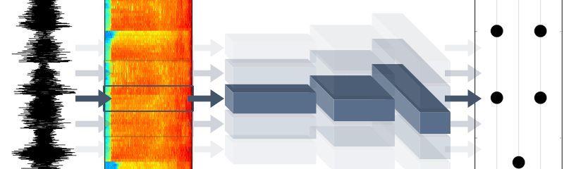
This article teaches you how to build a neural network that can recognize song types.
DataSet: This article uses the GTZAN Genre Collection music data set, address: [1]
This data set contains 1000 different songs, distributed in 10 different genres, 100 songs in each genre, and each song takes about 30 seconds.
Used library: Python library librosa, used to extract features from songs, and use Mel-frequency cepstral coefficients (MFCC).
The MFCC value imitates human hearing and has a wide range of applications in speech recognition and music type detection. The MFCC value will be directly input into the neural network.
Learn about MFCC
Let us illustrate MFCC with two examples. Please download Kick Loop 5[2] and Whistling[3] via Stereo Surgeon. One is the bass drum and the other is the high-pitched whistle. They are obviously different, and you can see that their MFCC values ​​are different.
Let's go to the code (all code files for this article can be found in the Github link).
The following is a list of content you need to import:
librosalibrary
glob, you need to list files in different types of directories
numpy
matplotlib, draw MFCC graphs
Keras sequence model, a typical feedforward neural network
Dense neural network layer, that is, a layer with many neurons.
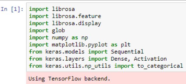
For example, unlike convolution, it has a 2D representation. You must use import activation, which allows you to provide an activation function for each neuron layer, and to_categorical, which allows you to convert the name of the class to such as rock, disco, etc., called one-hot Encode as follows:
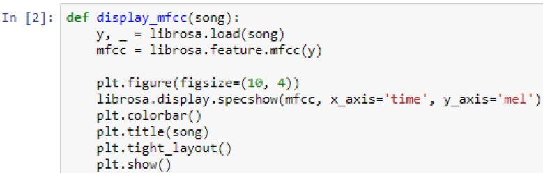
In this way, you have formally developed an auxiliary function to display the value of MFCC
First, load the song, and then extract the MFCC value from it. Then, use specshow, which is the spectrogram in the librosa library.
This is the pedal drum:
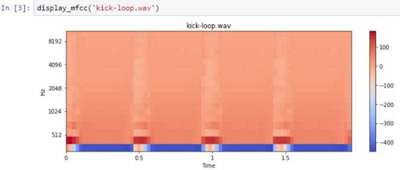
Low frequency: Kick loop5
It can be seen that the bass is very obvious at low frequencies. Not many other frequencies are represented. However, the spectrogram of the whistle sound obviously has a higher frequency representation:
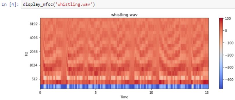
High frequency: Whistling
The darker or closer the color is to red, the greater the energy in that frequency range.
Limited song genre
You can even see changes in the frequency of the whistle. Here are the frequencies of disco songs:
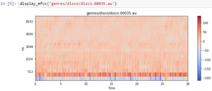
Song type/genre: Disco
The following is the frequency output:
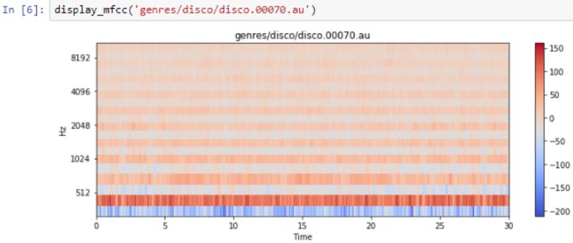
Disco Songs
You can see the beats in the previous output, but since they are only 30 seconds long, it is difficult to see individual beats. Comparing it with classical music, you will find that classical music does not have so many beats, but has a continuous bass line. For example, the following is the bass line from the cello:

Song genre: Classical
Here are the frequencies of hip-hop music:
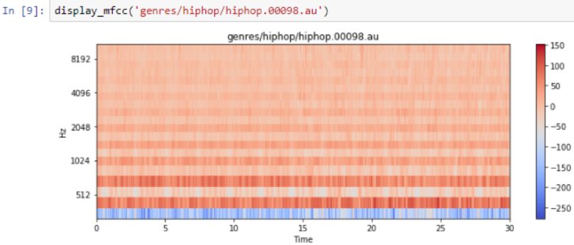
Song genre:HipHop
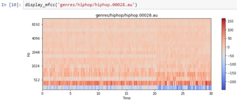
HipHop songs
It looks a bit like disco, and it is a neural network problem to distinguish the subtle differences between them.
There is another auxiliary function here, which only loads the MFCC value, but this time you are preparing for the neural network:
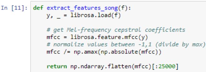
What is loaded at the same time is the MFCC value of the song, but since these values ​​may be between -250 and +150, they are not good for the neural network. You need to enter a value close to -1 to +1 or 0 to 1.
Therefore, it is necessary to calculate the maximum and absolute value of each song. Then divide all values ​​by the maximum value. In addition, the length of the song is slightly different, so only 25,000 MFCC values ​​need to be selected. You have to be very sure that the size of what you input into the neural network is always the same, because there are only so many input neurons, and once the network is built, it cannot be changed.
Limit songs to get MFCC value and genre name
Next, there is a function called generate _features_and_labels, which will iterate through all the different genres and all the songs in the data set, and then generate the MFCC value and the genre name:
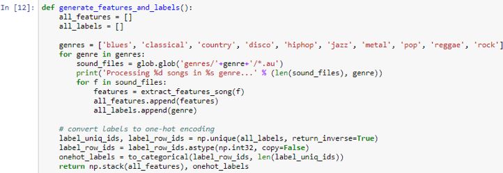
As shown in the screenshot above, prepare a list of all features and tags. Traverse all 10 genres. For each genre, check the files in that folder. 'generes /'+ genre +'/ *. The au' folder shows how the data set is organized.
When processing this folder, each file will have 100 songs; you can extract features and put these features in the all_features.append(features) list. The genre name of that song also needs to be listed in a list. Therefore, in the end, all features will contain 1000 entries, and all tags will also contain 1000 entries. In the case of all features, each of these 1,000 entries will have 25,000 entries. This is a 1000 x 25000 matrix.
For all the current tags, there is a 1000 entry list, which contains words such as blues, classical, country, disco, hip-hop, jazz, metal, pop, reggae, rock and so on. This is a problem, because the neural network does not predict words or predict letters. You need to give it a one-hot encoding, which means that every word here will be represented as ten binary numbers.
In the case of blues, it is 1 followed by 9 zeros.
In the classical (classical) case, 0 is followed by 1, followed by 9 zeros. And so on. First, use the np.unique(all_labels, return_inverse=True) command to return them as integers to calculate all unique names. Then, use to_categorical to convert these integers to one-hot encoding.
So, what is returned is 1000x10 dimensions. Because there are 1000 songs, each song has 10 binary digits to represent one-hot encoding. Then, use the command return np.stack(all_features) to return all the features stacked together, onehot_labels to a single matrix, and one-hot matrix. Therefore, call the upper function and save the features and labels:
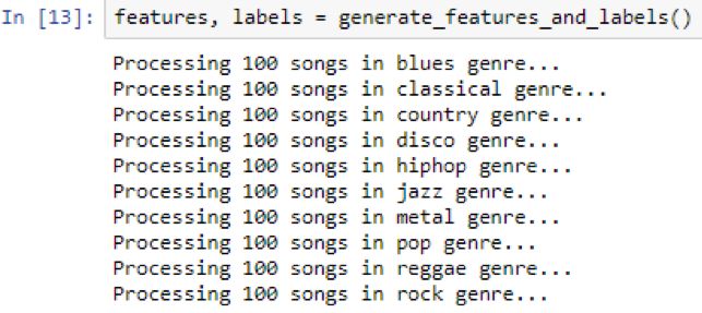
To make sure it is correct, please print the characteristics and the shape of the label as shown in the screenshot below. The characteristic is 1000×25000, and the label is 1000×10. Now, split the data set into a column and test the split. Define 80% of the marks as training_split = 0.8 to perform the split:
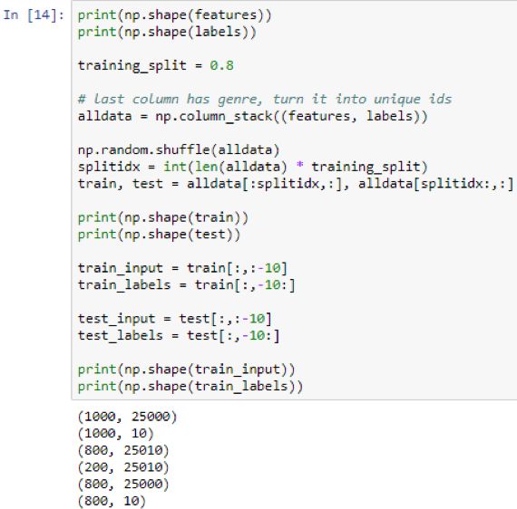
Next, build the neural network:
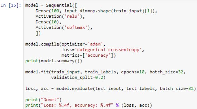
You will get a sequential neural network. The first layer is a dense layer of 100 neurons. In the first layer, you need to give the input size or input shape, in this example, it is 25000.
This indicates how many input values ​​each example has. 25000 will be connected to 100 in the first layer.
The first layer will perform a weighted summation of its input, weight and bias terms, and then run the relu activation function. relu means that anything less than 0 will become 0, and anything higher than 0 is the value itself.
Then, these 100 will be connected to the other 10, which is the output layer. The reason why it is 10 is because you have completed one-hot encoding and there are 10 binary numbers in the encoding.
The activation softmax used in the code tells you to take the output of 10 and normalize them so that they add up to 1. In this way, they eventually become probabilities. Now consider the one with the highest score or the highest probability among the 10 as the prediction. This will directly correspond to the highest number position. For example, if it is in position 4, then it is disco.
Next, compile the model, select an optimizer such as Adam, and define the loss function. Since you have multiple outputs, you may want to perform classification cross-entropy and measure accuracy so that in addition to the loss that is always shown, you can also see the accuracy during the evaluation. However, accuracy is more meaningful. Next, print model.summary, it will tell you detailed information about the layer. It looks like this:
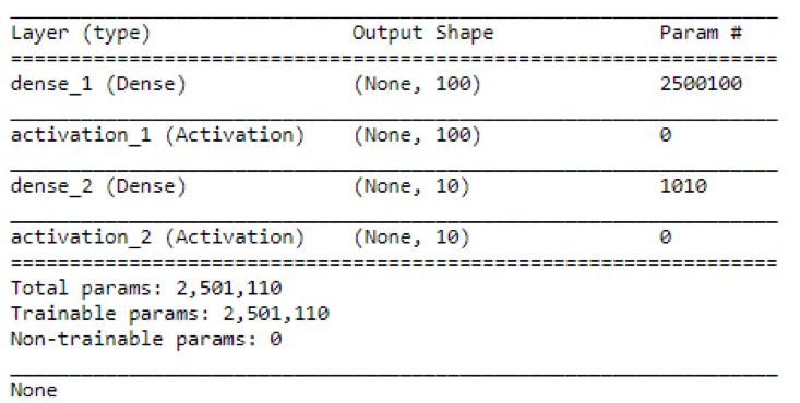
The output shape of the first layer of 100 neurons must be 100 values ​​because there are 100 neurons, and the output of the dense second layer is 10 because there are 10 neurons. So why does the first layer have 2.5 million parameters or weights? This is because you have 25,000 inputs.
You have 25,000 inputs, and each input goes into one of 100 dense neurons. Therefore, that is 2.5 million, and then add 100, because each of the 100 neurons has its own bias term, and its own bias weight also needs to be learned.
You have about 2.5 million parameters or weights. Next, run the fit. This requires training input and training labels, and get the number of epochs you want. You want 10, so repeat 10 times on the trained input. It needs a batch size to tell you this number. In this case, the song needs to be traversed before the weight is updated; and the validation_split is 0.2, which means that 20% of the training input needs to be received and split out. In fact, it is not correct. It trains and uses it to evaluate how well it performs after each epoch. In fact, the verification split has never been trained, but the verification split allows you to check the progress at any time.
Finally, because you have separated training and testing in advance, evaluate the test and test data, and print out the loss and accuracy of the test data. The following are the training results:
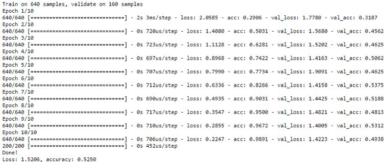
It prints while running, and always prints loss and accuracy. This is on the training set itself, not the validation set, so this should be very close to 1.0. You may not want it to be close to 1.0, because it may represent overfitting, but if you let it last long enough, it will usually achieve an accuracy of 1.0 on the training set because it remembers the training set.
What you really care about is the accuracy of the verification, which requires the use of a test set. The test set is data that has never been seen before, at least not for training. The final accuracy depends on the test data you separated in advance. Your accuracy is now about 53%. This may seem low, but be aware that there are 10 different genres. The accuracy of random guessing is 10%, so this is much better than random guessing.
Our Professional 10W solar panel manufacturer is located in China. including Solar Module. PV Solar Module, Silicon PV Solar Module, 10W solar panel for global market.

10W solar panel, PV solar panel, Silicon PV solar module
Jiangxi Huayang New Energy Co.,Ltd , https://www.huayangenergy.com